
Everyone knows a little something about circuits. People in the fields of computer engineering ought to know more: What is Boolean algebra, what is a physical circuit made of, what can digital circuits actually do and how to build large-scale systems out of combinational arrays of artfully simple logic gates. However, I personally strived for years asking myself questions like: Why do these circuits do what they claim to do, and why do people have to build modern computers utilizing them? What is a “computer”, exactly? And what’s the meaning for one to “program”, if anything?
I knew something about digital circuits and the rules of combinational logic underlying them. I also knew a few paradigms of programming and how to solve problems using practical languages (math sketches on pen & papers, C, Java, Python, ML, ….). I have even heard about the fantastic Turing machine and the dreadful halting problem – like many programmers do. What I don’t know yet is how our logic and language interplayed, and how they codefined the limitation of computation; needless to say, there is still a missing chain from all the logic and mathematical theories as well as all the languages (either human natural, semi-formal or formal) I have learned so far, to a real-world computer which can do some fancy stuff (while it can’t do some others efficiently or even at all), that I have yet to complete.
Here I begin, trying to learn a “big picture” of Computer Science, in a hopefully intuitive way: Not on how to write a program that merely works (that would be the job of an engineer), but rather on how to argue when programs work and when they don’t, so well as to argue about fundamental issues like “You can’t solve this problem with a program efficiently” or “You just can’t solve this kind of problem at all, no matter how hard you tried!”.
1 An Informal Discourse of Computation
As a common ground that we agree on, anything written in a language (natural languages like English, programming languages like Java, or even nonlinear notations like in math and logic) may be encoded as bit-strings, which are merely sequences of 0 and 1s, in some way. Even the most intractable, unsolvable problem, may be encoded into a bit-string so well as the easiest ones. If we ever find any solution(s) to that problem, we encode them into bit-strings as well.
So, how do we define a computation, in terms of these sequences of 0 and 1s that represent a problem and its valid solution(s)? Easily, a computation is but a mapping: \[\mathcal{C} : \mathcal{L}_\mathsf{problem} \to \mathcal{L}_\mathsf{solutions}\] where language \(\mathcal{L}_\mathsf{problem}\) is the problem space, and language \(\mathcal{L}_\mathsf{solutions}\) is the power set of the solution space (since a problem can have either zero, exactly one or more solutions).
Intuitively, if we want to solve the problem “\(1 \times 2 = ?\)”, and assume that we encode the arithmetic expression as an ASCII string (‘\(1\)’ as 00110001, ‘\(\times\)’ as 00101010, ‘\(2\)’ as 00110010, respectively), we could construct a mapping \(\mathcal{C}\) such that \[\mathcal{C} : \mathtt{00110001\,00101010\,00110010} \mapsto \mathtt{00110010}\]
Of course, this is just an abstract model of computation that, according to our fixed “protocol” of problem encoding, outputs the solution of \(1 \times 2\) correctly. Nothing more. One can implement this mapping trivially. But if we want to define a computation that does multiplication correctly for every pair of 1-digit integers, we need to have more “mapping rules” like \[\mathcal{C} : \mathtt{00110001\,00101010\,00110010} \mapsto \mathtt{00110010}\] \[\mathcal{C} : \mathtt{00110001\,00101010\,00110011} \mapsto \mathtt{00110011}\] \[\mathcal{C} : \mathtt{00110001\,00101010\,00110100} \mapsto \mathtt{00110100}\] \[\cdots\] which say \(1 \times 2 = 2\), \(1 \times 3 = 3\), \(1 \times 4 = 4\), etc.
This would be exhausting, wouldn’t it? If you are a programmer, you are telling your computer to memorize the whole multiplication table this way. Certainly this is not what we do in reality, otherwise we as programmers need to enumerate every possible case of problems, find their solutions and encode all of them into computers through enormous human labor. So our naïve thinking of approaches for “computation” doesn’t really work. The intuition tells us that an ideal computer should do much better than this, with some “magic” that automatizes the process of finding solutions. Implementing such a computer would be nontrivial, but the whole point of building a computer is that we don’t know the answers to some problems yet and we want the computer to solve them for us!
Here comes the big question now: Is every problem in a given language \(\mathcal{L}_\mathsf{problem}\) solvable? Or, more technically, can we generally build a computer that for each problem input, always outputs its solutions in finite time?
To simplify our problem a little bit (excuse the pun here), let us consider first a problem with a deterministic solution consisted of only a single bit. Such problems are often called decision problems, for their solutions are merely yes-or-no answers, e.g., Is that integer a prime? Is that real number rational? Is this theorem valid/provable? Does that computation process ever terminate? Does my own computation (that tries to solve the meta-problem of termination) terminate? Decision problems are not only of theoretical importance, but they also constitute solutions for any arbitrary problem: For example, is the first bit of the encoded solution of \(1 \times 2\) equal to \(0\)? Is the second bit of the encoded solution of \(1 \times 2\) equal to \(0\)? Keep proposing decision problems like that, then we get a multi-bit solution for any problem as we desired. In other words, any arbitrary problem is reducible to a sequence of decision problems. Therefore, the notion of computation (on decision problems) is simplified as a mapping: \[\mathcal{C} : \mathcal{L}_\mathsf{problem} \to \Sigma\] where \(\Sigma = \{0,1\}\).
So, we have now reduced the big question to: Given a language \(\mathcal{L}_\mathsf{problem}\), does there exist a model of computation (which is just a fancy word for an “ideal computer”) that always outputs a single-bit answer \(b \in \Sigma\) for any problem \(p \in \mathcal{L}_\mathsf{problem}\)?
Later on we tend to ask ourselves this very question again and again, in dissimilar scopes of “languages”, until we realize the self-evident fact that this question itself is expressible in certain \(\mathcal{L}_\mathsf{problem}\), so that we are tempted to treat it like a decision problem and ask whether an ideal computer can solve it. That would ultimately put an end to our abilities of computation, as shown by the undecidability of the halting problem (Turing 1937). However, undecidability implies that the language \(\mathcal{L}_\mathsf{problem}\) must be a very powerful one such that a problem can state itself (as powerful as a natural language like English). That may look a little too metaphysical so far, therefore we start by restricting our language \(\mathcal{L}_\mathsf{problem}\) to a finite set, that is, we can say only a finite number of things in this language:
Definition 1. (Finite language) A finite language \(\mathcal{L}\) is a finite set of strings \(\Sigma^k\) (where \(0 \leq k \leq n\)).
Finite languages are a very restricted form of languages; there is no way to construct arbitrarily long strings using grammars in such languages: Think of a little baby who just learned three words “mama”, “papa” and “pee”, then these are all she could say. Samely, we can ask “simple” one-shot questions like “Is 0 an even number?” “Is 42 an even number?”, but not “If \(n \in \mathbb{N}\), is \(6n\) an even number?”, because it would be impossible to formulate the notion of general natural numbers (although countably infinite) in this kind of language.1
Within our restricted finite language \(\mathcal{L}\), we can give an initial attempt to define computation and computability:
Definition 2. (Computation in a finite problem space) A computation in a finite problem space is a mapping \[\mathcal{C} : \mathcal{L}_\mathsf{problem} \to \Sigma\] where \(\mathcal{L}_\mathsf{problem}\) is a finite language, and \(\Sigma = \{0,1\}\).
A problem \(p \in \mathcal{L}_\mathsf{problem}\) is said to be computable if and only if \(\mathcal{C}\) is total.
Let’s ask the same old question here again: Given a finite language \(\mathcal{L}_\mathsf{problem}\), is every problem \(p \in \mathcal{L}_\mathsf{problem}\) computable? Or, is there a model of computation that always “decides” the answer for every possible input?
By definition, yes, there is, as long as \(\mathcal{C}\) is totally defined! If we are able to enumerate all problems in the finite language \(\mathcal{L}_\mathsf{problem}\), we can then pre-compute their solutions using other methods and plant these problem-solution pairs into our model. So our model can be simply a lookup table that outputs a certain yes-or-no answer (\(0\) or \(1\)) for each possible input (abstract problem). This is much the same as our previous naïve approach for computation, except that this time we are using it to demonstrate what we can do, without caring much about how we do things efficiently. We can easily convince ourselves that our model of computation, if correctly constructed, must be sound; since every problem in the finite language is decidable, our model of computation, if totally constructed, must also be complete.
Thus, we have shown that computation in a finite problem space can be implemented, soundly and completely, by a model of computation, that we are yet to construct.
Before we start constructing our first model of computation, we need to rethink of our notions of “problems and their solutions” very carefully, in an epistemological way. As we said before, we could just “pre-compute their solutions using other methods and plant these problem-solution pairs into our model”, but if we don’t know the solutions yet, are we still able to compute? In many cases we are, e.g., checking whether a large number is prime, or proving the four color theorem, where we plant axioms and derivation rules, instead of the actual solution itself, into the model of computation. However, there are also many problems that cannot be solved in any way (in a mathematical sense, at least), and their unsolvability clearly implies non-computability. They are worth some elaboration here:
- Consider a problem of determining the state of a subatomic particle prior an observation. Quantum mechanics claims that this decision problem cannot have a simple yes-or-no answer, unless an observation is done and the wave function collapses to a single eigenstate. Since we cannot solve such a problem due to physical properties, we would not expect to solve them by any computer. These problems are naturally unsolvable; they are a reflection that our knowledge about the physical world is naturally bounded, thus they are destined to be non-computable.
- Consider a problem of deciding the truth or falsity of “This statement is false”, which is the well-known liar paradox. Human languages are so powerful that they are allowed to have self-referencing terms and enumerate on them, and if we insist on logic consistency (soundness), problems like this are undecidable either. Another example is the halting problem, i.e., “Does there exist a program that determines whether an arbitrary program terminates?” Such problems are paradoxical unsolvable. If we ever construct something to solve problems in unrestricted languages, we end up with an incomplete model of computation2, because there are always problems that can never be computed. Fortunately, in our extremely restricted form of finite language \(\mathcal{L}_\mathsf{problem}\), we are still far from that level of undecidability, as self-referencing terms are excluded from our finite language (otherwise if we ever try to write down all the problems in the language iteratively, it would propagate an infinite hierarchy of problems and \(\mathcal{L}_\mathsf{problem}\) would be infinite then) and we can reasonably argue that our model of computation is complete and every problem can be computed.
In the following sections, we will show that (1) Boolean circuits constructed from a minimal set of logic gates are sufficient to accommodate any computation \(\mathcal{C}\) as we just defined, for every mapping from the finite language \(\mathcal{L}_\mathsf{problem}\) to \(\Sigma\), as a complete model of computation; (2) In spite of that, a Boolean circuit is, in fact, a relatively weak (arguably the weakest) model of computation, due to the restriction we set on the language it recognizes. By gradually enriching our language (from expanding the problem space infinitely to allowing recursive terms), we will be able to state more and more interesting problems and compute them by constructing abstract machines that are more powerful than a primitive Boolean circuit, and, eventually, we will have grown a language that is so rich that some statements cannot even be decided by any ideal abstract machine, as a consequence of Gödel’s incompleteness theorem (Gödel 1931).
2 Finite Language and Boolean Circuits
Recall that we defined a computation (of a decision problem) as a mapping \[\mathcal{C} : \mathcal{L}_\mathsf{problem} \to \Sigma\] where \(\mathcal{L}_\mathsf{problem} \subseteq \{\Sigma^k | \Sigma = \{0,1\}, 0 \leq k \leq n\}\) and \(\Sigma = \{0,1\}\).
Although the output is one single bit \(b \in \Sigma\), we can reduce any problem of output size \(\ell\) to a finite sequence of decision problems \(\mathcal{C}_1, \mathcal{C}_2, \dots, \mathcal{C}_\ell\) and concatenate their outputs together as bit-string \(b_1 b_2 \dots b_\ell\). Therefore the computability of a decision problem is the most essential for us.
We have also shown that if the mapping \(\mathcal{C}\) is totally defined, then there exists a model of computation that decides all problems in the language completely. Now we want to construct that model, in a physically implementable way.
Intuitively, since all problems in a finite language can be enumerated, why not just build a lookup table as our first model? Such a naïve approach is of theoretical importance, but, as we discussed before, that requires us as programmers to enumerate every possible case of problems, find their solutions and encode all of them into computers through exhausting human labor; furthermore, that would make our computation much more like reading a handbook rather than actually computing anything.
a.k.a. Abramowitz and Stegun. (Source: Wikimedia. Photographed by agr.)
If the language we use to describe problems allows at most \(n\) bits, we can have as many as \(2^n\) questions whose answers must be contained in the lookup table. \(2^n\) is an exponentially large number, so it’s unlikely to be as easy as browsing a handbook in reality; it could be like traversing a Library of Babel!
There might be mechanized ways to support our searching in the table, but they won’t scale well because the table is inherently large: No matter in which way you look up in a table, it still has to record as many as \(2^n\) entries, frustratingly. So we must come up with smarter models of computation, rather than give up easily on computers with such an exponentially growing level of time/space complexity.
It would be helpful to think of our so-called computation as a black box:
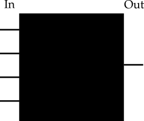
Although we do not know how this black box works internally yet, we can tell that it takes a finite number of (at most) \(n\) input bits; it outputs a single bit; it is deterministic, so it always outputs the same bit when given same input; it is stateless, so it cannot read from or write to any “memory”, nor is it allowed to access an external device during a computation or across multiple computations. Given these a little overly simplified properties, one could easily assume that there is something like a “circuit” in the black box, which does certain kind of magical stuff to compute that single bit.
Digital circuits are exactly the first model of computation we are going to talk about. More precisely, pure Boolean circuits.
Boolean circuits can be described as a combination of logic gates. Let’s briefly review some basic ones of them, semi-formally:
- NOT gate is a mapping \(\lnot : \Sigma \to \Sigma\) that outputs 1 iff the input bit is 0, otherwise outputs 1.
- AND gate is a mapping \(\land : \Sigma \times \Sigma \to \Sigma\) that outputs 1 iff both input bits are 1, otherwise outputs 0.
- OR gate is a mapping \(\lor : \Sigma \times \Sigma \to \Sigma\) that outputs 1 if either input bits is 1, otherwise outputs 0.
- XOR gate is a mapping \(\oplus : \Sigma \times \Sigma \to \Sigma\) that outputs 1 iff exactly one input bit is 1, otherwise outputs 0.
- NAND gate is a mapping \(\uparrow : \Sigma \times \Sigma \to \Sigma\) that outputs 1 iff no more than one input bit is 1, otherwise outputs 0.
- NOR gate is a mapping \(\downarrow : \Sigma \times \Sigma \to \Sigma\) that outputs 1 iff no input bit is 1, otherwise outputs 0.
We have \(2^{2^1}=4\) different logic gates with 1-bit input (they are the identity gate that outputs the input, the NOT gate that reverses the input, the gate that always outputs 0, the gate that always output 1), \(2^{2^2}=16\) different logic gates with 2-bit input, \(2^{2^3}=256\) different logic gates with 3-bit input. If the size of our problem is \(n\) and we insist on building a circuit with a single big logic gate, then we would have \(2^{2^n}\) different choices of gates – each of which corresponds to a whole lookup table containing \(2^n\) entries.
Luckily, we won’t need that googolplex-like number of logic gates with too many input bits to implement our model of computation at all, as justified by the following claim:
Claim 3. Logic gates with 2-bit input are sufficient to cover the functionalities of any gates.
We show this by reduction: A gate with \(n\) (\(n \geq 2\)) input bits is replaceable by 2-bit gates if and only if any gate with \(n-1\) input bits is replaceable by 2-bit gates, so that we can construct a gate consuming the first \(n-1\) input bits and replace it with its equivalent set of 2-bit gates, then take its output and the \(n\)-th input bit into a finalizing 2-bit gate. When \(n = 2\), this replaceability holds trivially.
On the other hand, a gate with 1 input bit is easily replaceable by 2-bit gates, since we can use the same input bit twice as the input of a 2-bit gate.
■
Claim 4. Logic gates with 1-bit input are not sufficient to cover the functionalities of some gates.
Assume that any logic gate is replaceable by 1-bit gates. Let’s take an AND gate and replace it by some set of 1-bit gates. The output bit is the output of a 1-bit gate, thus it must be either the same as one of input bits, the reverse of one of input bits, 0 in all cases or 1 in all cases. By checking the truth table of the AND gate, we conclude that none of them is the case. That is a contradiction.
■
Some questions remain. (1) We have merely shown that logic gates with 2-bit input (possibly combined with 1-bit gates for technical convenience) are sufficient to implement the logic of any digital circuits. But are they sufficient to simulate our defined computation \(\mathcal{C} : \mathcal{L}_\mathsf{problem} \to \Sigma\)? If we are not able to argue that, then we cannot convincingly say this is the right model of computation we are looking for. (2) Do we need all these \(2^{2^2}=16\) logic gates with 2-bit input to build a circuit that performs our computation? Less is more, a theory/model composed of a minimal set of axiomatic components is often the most desirable.
Claim 5. For every computation \(\mathcal{C} : \mathcal{L}_\mathsf{problem} \to \Sigma\), there exists a Boolean circuit that simulates it.
We show this by induction. For input \(\varepsilon \in \mathcal{L}_\mathsf{problem}\), the statement holds vacuously.
For input \(p \in \Sigma^1 = \{0,1\}\), to get the output bit \(b \in \Sigma\) we desired, we construct a Boolean circuit \(C_1\) using a 1-bit gate.
Assume that for any input \(p' \in \Sigma^i\), we already have a circuit \(C_i\) that simulates its computation. For input \(p \in \Sigma^{i+1}\), we construct \(C_i\) taking the first \(i\) bits as input, then construct a finalizing circuit \(C_{i+1}\) using a 2-bit gate, which consumes the output from \(C_i\) and the last remaining bit. By induction, we construct a Boolean circuit \(C_{i+1}\) (using only 1-bit and 2-bit gates) that simulates computation \(\mathcal{C}\).
■
Claim 6. For every computation \(\mathcal{C} : \mathcal{L}_\mathsf{problem} \to \Sigma\), there exists a Boolean circuit using only AND gates and NOT gates that simulates it.
This is a stronger statement than Claim 5, but since we have argued that Claim 5 is true, the only thing left to be shown is that any Boolean circuit composed of arbitrary logic gates can be replaced by some other circuit composed of only AND gates and NOT gates. Furthermore, by Claim 3 we know that any arbitrary logic gate is reducible to a combination of 2-bit gates, so we only need to show that every 2-bit gate can be simulated using only AND gates and NOT gates.
There are only \(2^{2^2}=16\) possible logic gates with 2-bit input, so we could just complete the proof case by case: Try to come up with something composed of only AND gates and NOT gates, then verify that its truth table is equivalent to the one of the original logic gate.
| # | Logic gate with 2 input bits (\(x\) and \(y\)) | Truth table encoded | Synonyms/Aliases |
|---|---|---|---|
| 0 | \(x \land \lnot x\) (alternatively, \(y \land \lnot y\)) | 0000 |
\(\bot\) contradiction |
| 1 | \(x \land y\) | 0001 |
conjunction (AND) |
| 2 | \(x \land \lnot y\) | 0010 |
\(x \not\to y\) \(x \not\supset y\) \(\lnot(x \to y)\) \(\lnot(x \supset y)\) nonimplication abjunction |
| 3 | \(x\) | 0011 |
identity of \(x\) |
| 4 | \(\lnot x \land y\) | 0100 |
\(x \not\leftarrow y\) \(x \not\subset y\) \(\lnot(x \leftarrow y)\) \(\lnot(x \subset y)\) converse-nonimplication |
| 5 | \(y\) | 0101 |
identity of \(y\) |
| 6 | \(\lnot(\lnot x \land \lnot y) \land \lnot(x \land y)\) | 0110 |
\(x \oplus y\) \(x \not\leftrightarrow y\) \(x \not\equiv y\) exclusive disjunction (XOR) |
| 7 | \(\lnot(\lnot x \land \lnot y)\) | 0111 |
\(x \lor y\) disjunction (OR) |
| 8 | \(\lnot x \land \lnot y\) | 1000 |
\(x \downarrow y\) negation of disjunction (NOR) |
| 9 | \(\lnot(\lnot(\lnot x \land \lnot y) \land \lnot(x \land y))\) | 1001 |
\(x \leftrightarrow y\) \(x \equiv y\) biconditional equality (XNOR) |
| 10 | \(\lnot y\) | 1010 |
negation of \(y\) |
| 11 | \(\lnot(\lnot x \land y)\) | 1011 |
\(x \leftarrow y\) \(x \subset y\) converse-implication |
| 12 | \(\lnot x\) | 1100 |
negation of \(x\) |
| 13 | \(\lnot(x \land \lnot y)\) | 1101 |
\(x \to y\) \(x \supset y\) implication |
| 14 | \(\lnot(x \land y)\) | 1110 |
\(x \uparrow y\) negation of conjunction (NAND) |
| 15 | \(\lnot(x \land \lnot x)\) (alternatively, \(\lnot(y \land \lnot y)\)) | 1111 |
\(\top\) tautology |
With 2 input bits (\(x\) and \(y\)) and 2 elementary logic operators (\(\land\) and \(\lnot\)), we can construct infinitely many 2-bit Boolean expressions, but the possibility of their truth tables is finitely bounded (to \(2^{2^2} = 16\)). If two expressions yield the same truth table, we consider their corresponding logic gates as equivalent (and we can replace one by another, usually its simplest form).
■
By Claim 5 and Claim 6, we are now convinced that Boolean circuits, as our very first model of computation, are capable of the computation \(\mathcal{C}\) for a finite language as we defined. Claim 6 further says that AND gates and NOT gates are sufficient to construct Boolean circuits for any computation, so even though we have \(2^{2^1}=4\) types of 1-bit gates and \(2^{2^2}=16\) types of 2-bit gates, if we choose the correct functionally complete (or expressive adequate) set, i.e., \(\{\land, \lnot\}\), two types of gates are sufficient. Using the same technique we applied when justifying Claim 6, we may prove that \(\{\lor, \lnot\}\) is also a functionally complete set. Even better, we have that \(\{\uparrow\}\) (“Sheffer stroke”), even though it’s a singleton of NAND gate, is also a functionally complete set that is sufficient to implement any Boolean circuits; so is \(\{\downarrow\}\) (“Peirce arrow”), the singleton of NOR gate. There is a deeper reason for this (Pelletier, Martin, and others 1990), but I won’t go into details since neither logic nor Boolean algebra is my main topic here.
Notice that, Claim 6 justifies that there exists a Boolean circuit for every computation, but it does not provide much clue for constructing such a circuit for a specific computation. However, for most of us this is no rocket science: Given an arbitrary truth table, we write down its disjunctive (or conjunctive) normal form, (optionally) simplify it and rewrite it using prescribed functionally complete set of logic gates (\(\{\land, \lnot\}\), in our case). See a concrete example:
| \(x\) | \(y\) | \(z\) | Output \(b\) |
|---|---|---|---|
| 0 | 0 | 0 | 1 |
| 0 | 0 | 1 | 0 |
| 0 | 1 | 0 | 0 |
| 0 | 1 | 1 | 0 |
| 1 | 0 | 0 | 1 |
| 1 | 0 | 1 | 0 |
| 1 | 1 | 0 | 0 |
| 1 | 1 | 1 | 1 |
(In most engineering treatments, notations like \(\bar{x}\bar{y}\bar{z} + x\bar{y}\bar{z} + xyz\) are commonly used, but in commutative algebra the operator “\(+\)” has a different meaning that is analogous to XOR rather than OR, so we stick with the conventional logic symbols here.)
The best thing about Boolean circuits is that people can implement arbitrary computation with finite input by building up sophisticated combination from only a minimal set of elementary logic gates so that the production of such circuits can be industrialized – that’s why this model is sometimes called combinational logic, although digital circuits may be used for performing many general-purpose computing tasks rather than just representing “logic”. However, there is a price to pay beneath their designs: By allowing only logic gates from a minimal set, the complexity of circuits grows progressively. Reducing the number of gates required and optimizing the size of the circuit are engineering problems, but from a theoretic perspective, they are inherently hard – there is a bunch of circuit complexity classes and related theories that study them. It was proved that a general computation involving \(n\) input bits requires Boolean circuit of size \(\Theta\left(\frac{2^n}{n}\right)\) (Shannon and others 1949), but it is not known whether a specific computation \(\mathcal{C}\) has a superpolynomial lower bound for the sizes of corresponding Boolean circuits.
Why are some circuits so complex? Because computation can be hard. We can think of this unavoidable intractability in an alternative way: Computation for a finite language is trivial by using a lookup table (which can be seen as an equivalent model of computation); deciding a finite language with length \(n\) requires at most \(2^n\) entries in the lookup table for a total mapping, assumed that this mapping (of computation) is completely random. Sometimes we can find a “pattern” in the computation, so we don’t need the whole exponentially large table to look at – we can do a lookup in a polynomial or even constant-size sub-table and decide the language efficiently. Sometimes we can’t: There are still many computationally hard problems, if we could ever write down a lookup table for its problem-solution mapping, the solutions will narrate complete pseudorandomness (Just think of a decision problem like “Generate a random bit from any input”). If we try to convert the lookup table to its equivalent Boolean circuit, or even simulate the computation using a much more advanced model (e.g., Turing machine, x86 instructions, programming in Java, …), easy problems are still easy3, while hard problems will always be hard, because our choice of model of computation will not essentially change the algorithmic hardness of a problem; it only changes our view of dealing with that problem.
As shown by the above thought experiment, there is often a trade-off between certain complexities: Either we have a big lookup table that exhausts time and space, or we try to build up a circuit with a great deal of wires and gates. But the most important conclusions we reached in this section, are that (1) Finite language corresponds to the simplest form of computation; (2) If we can state a problem in a finite language, then it is decidable (logically); (3) Decision problems for finite languages can be solved by Boolean circuits, our first model of computation; (4) Boolean circuits can be constructed using a minimal set of logic gates, e.g., AND gates and NOT gates.
3 Information Towards Simulation
Before finishing the introduction to the first model of computation, we recap by some fundamental (but inspiring) questions:
- Is our model of computation sound? In other words, does it correctly simulate the computation \(\mathcal{C}\)?
Yes. Boolean circuits are sound by construction, as long as Boolean algebra is deterministic.
- Is our model of computation complete? In other words, can it simulate every computation \(\mathcal{C}\) (by deciding a finite language \(\mathcal{L}_\mathsf{problem}\))?
Yes. As argued by Claim 5. So far as the mapping of computation \(\mathcal{C}\) is total, we can always construct a Boolean circuit that decides the finite language \(\mathcal{L}_\mathsf{problem}\).
- What is the limitation of Boolean circuits? In other words, what kinds of computation is it incapable to simulate?
It wouldn’t be too hard to see the fatal issue about Boolean circuits: They only take finite inputs. So if we have a language containing an unbounded number of strings, no Boolean circuit will ever be able to decide it, let alone doing any useful computation. However, even if we consider only finite languages, a fixed Boolean circuit still has a bounded ability for computation. We show that by proposing some more questions.
- Does there exist a Boolean circuit that simulates the computation of every possible Boolean circuit?
No. This is an easy question, since “the set of all Boolean circuits” is infinite (I would also argue that it’s also countably infinite), and clearly the set of all finite languages is also infinite. As a fun way of informal thinking, if there is such an omnipotent Boolean circuit that can simulate every other circuit, someone would already have patented it and earned a deserved fame. Certainly this would not happen!
- Does there exist a Boolean circuit with \(n+1\) input bits that simulates the computation of a Boolean circuit with \(n\) input bits?
Yes, there is. Our new Boolean circuit should work like this: Take the first \(n\) bits, replicate the original Boolean circuit with \(n\) input bits that we already have, and use that one’s output as its output. Our constructed circuit also takes an extra bit, but that doesn’t matter and can be safely dropped; if we must use it, we could use it to construct a \(\top\) and put the output bit and the original circuit together with an AND gate.
- Does there exist a Boolean circuit with \(n\) input bits that simulates the computation of a Boolean circuit with \(n+1\) input bits?
Intuitively, one would say no, because there is no way for a circuit with only \(n\) input bits to accommodate for \(n+1\) input bits. But that reasoning can be hard to justify – What if we just construct a circuit, sending the extra input bit to a null device as a “dumb” placeholder? How would you argue that it can never do the computation as the original circuit does? In fact, there is an obvious counterexample: If a Boolean circuit with \(n+1\) input bits implements a tautology (i.e., always outputs 1), then it surely can be simulated by a Boolean circuit with \(n\) input bits, because we don’t expect an extra bit to offer any more useful “information” for this computation.
Whenever we fail to justify something convincingly, a new theory emerges. Information theory is the one we are looking for.
The information entropy (Shannon entropy) of a random variable \(X\) is defined as (Shannon 1948) \[\operatorname{H}(X) = -\Sigma_{x \in \mathcal{X}} p(x) \log p(x)\]
Given a Boolean circuit of input size \(n\), consider its equivalent lookup table which contains \(2^n\) entries of solutions to corresponding decision problems. We need a \(2^n\)-bit string to encode this table. Let \(X\) be this \(2^n\)-bit string.
What does information theory tell us? If we already know with certainty that every problem in our finite language \(\mathcal{L}_\mathsf{problem}\) has answer \(1\) (tautology), then our encoded lookup table would be the string \(x = \underbrace{11\cdots1}_{2^n\ \textrm{1s}}\). There is no point of computing here (since the answer is assumed a priori), and since \(p(x) = 1\), we get the entropy of this lookup table \(\operatorname{H}(X) = 0\), that is, this “computation” does not provide any extra information of our interest.
The usefulness of computation dramatically emerges when we are not sure about the answers. If we know that every problem in our finite language \(\mathcal{L}_\mathsf{problem}\) has exactly the same answer, but we don’t know what it is (that we must find out), then our encoded lookup table would be either \(x_0 = \underbrace{00\cdots0}_{2^n\ \textrm{0s}}\) or \(x_1 = \underbrace{11\cdots1}_{2^n\ \textrm{1s}}\). Since we have no a priori knowledge about the universal answer, we would not assert which version of lookup table is more likely be yielded by computation. Thus, it is natural to assume that \(p(x_0) = p(x_1) = \frac{1}{2}\). The entropy of this lookup table is \(\operatorname{H}(X) = -(p(x_0)\log_2 p(x_0) + p(x_1)\log_2 p(x_1))\) = 1, that is, this computation can provide as much information as exactly 1 bit (or “1 shannon”, to emphasize the fact that this is a measure of information entropy), even though its lookup table contains strings of \(2^n\) bits.
In most interesting computations, we have no idea how the problem space \(\mathcal{L}_\mathsf{problem}\) is related to the solutions at all, and the encoded lookup table, in the scope of our a priori knowledge, is a uniformly random string. Practically we are unable to enumerate all its possibilities, but we can still assume that given all \(2^n\) entries, each of which has a fair probability of being 0 or 1, then a probable lookup table appears with probability \(p(x) = 2^{-2^n}\). The entropy of this lookup table is \[\operatorname{H}(X) = -2^{2^n} \cdot 2^{-2^n} \log_2 2^{-2^n} = 2^n\]
This is an interesting result. It shows that as our input size (in the finite language \(\mathcal{L}_\mathsf{problem}\)) increases, the information provided by the naïve “lookup table approach” of computation booms exponentially, assuming that we have no a priori knowledge on how to do the computation efficiently. Notice that this is merely a theoretical upper bound; in reality, if we can ever build a Boolean circuit to decide a problem so that we do not have to use a lookup table, then we already have found some “pattern” in the computation thus our model of computation would not have included so much useful information (as an exponentially large lookup table).
With the notion of information entropy, we can argue about the statement we made before: The information contained in a Boolean circuit with \(n\) input bits has an upper bound of \(2^n\) bits (which is equivalent to a lookup table model), but a Boolean circuit with \(n+1\) input bits can carry as much information as \(2^{n+1}\) bits. Thus, it is generally impossible to simulate any Boolean circuit with \(n+1\) input bits using a circuit with equal to or less than \(n\) bits. Although in some special cases we can, e.g., imagine a circuit with \(n+1\) input bits but only carries an information entropy of \(2^n\), then the simulation should be tractable for an \(n\)-bit circuit; moreover, if a big circuit always outputs either “0” or “1” for any problem in the language, then it can be simulated easily by a nontrivial circuit, since its information entropy is merely \(1\) bit.
Clearly, the ability of a model of computation to simulate one another is restricted by the information it maintains. Thus, we can sketch a hierarchy for all Boolean circuits: any 1-bit circuit can be simulated by a 2-bit circuit, any 2-bit circuit can by simulated by a 3-bit circuit, …, any \(n\)-bit circuit can be simulated by a \((n+1)\)-bit circuit, but generally not contrariwise.
Thinking about this hierarchy intuitively, we would conclude that every Boolean circuit with more input bits \(n\) (corresponding to a larger finite language \(\mathcal{L}_\mathsf{problem} \subseteq \{\Sigma^k\ |\ 0 \leq k \leq n\}\)) has a stronger ability of computation than its predecessors. As this chain goes forever, a Boolean circuit with \(\infty\) input bits would have the ultimate ability to decide any finite language (thus it can simulate every other Boolean circuit), which cannot be achieved because we can never build such a circuit of infinitely many input bits in reality. Therefore, there is no such model that we can use to decide problems in an “infinite” language. Is that true?
In a way, yes. Remember that our choice of model of computation will not essentially change the algorithmic tractability of a problem, so if a problem asks for an impossible decision on arbitrary, recursively large things, we just cannot solve it, no matter from which model of computation we seek for help. However, if a problem asks for some decisions on very specific things, e.g., Does the string “a” consist of only letter a? Does the string “aaa” consist of only letter a? Does the string “aaaba” consist of only letter a? We can immediately tell that there is a general mechanizable way of deciding it, regardless of the length of the questioned string. Such a language \(\mathcal{L}_\mathsf{problem} = \{\Sigma^k\ |\ k \in \mathbb{N}\}\) is infinitely large but every problem defined by it is decidable; as it’s not even a finite language we can’t build a Boolean circuit for it, that doesn’t mean we can’t solve it! The implication is that we would miss out so much between finite languages and arbitrarily infinite languages4, if we just restrict our mindset to finite languages and pure Boolean circuits that recognize them.
What we have achieved so far, is to argue that Boolean circuits are a sound and complete model of computation for deciding finite languages, with all the reasoning done in two powerful arbitrarily infinite languages: English as an ambiguous, informal natural language; and mathematics as a less ambiguous, semi-formal symbolic language. Naturally, we would think that it is feasible to describe and reason about a language via a more expressive one, as well as to simulate a model of computation using a more powerful one. We will demonstrate this in the next section: First we formalize our model of computation (Boolean circuits), with its syntax defined as a context-free grammar. Then we simulate the computation of Boolean circuits using total functional programming, by implementing it as an embedded domain-specific language. Lastly, we show the semantic equivalence of two programs (combinational circuits), using notions from deductive logic. All these approaches correspond to something in between finite languages and arbitrarily infinite languages; they have sufficient power for formalizing Boolean circuits, our first simple model of computation.
4 Formalizing Combinational Logic
In Section 1 we introduced finite languages, as the simplest representing form of computation. In Section 2 we demonstrated that Boolean circuits, as a model of computation, may be used to decide finite languages, although it can carry an exponential level of complexity in worst cases. Building a circuit physically may be challenging, but simulation (either by a bigger circuit or by a more powerful model of computation) of them is possible, as we concluded in Section 3.
To enable ourselves some formal thinking, and for practical reasons, to simulate this model on a computer, we must eliminate any ambiguity and present our precise ideas in a symbolic way. The finite language we defined in Section 1 is already a formal language, but the model of computation which decides it, that is, Boolean circuits, is not formalized by us yet. Thinking of it as a minimal programming language, we may describe our model formally with regards to two supporting components: its syntax and its semantics. Both are critical components for any concrete implementation of a model of computation.
4.1 Syntax
Visually, Boolean circuits are planar structures. In order to give a formal description of a circuit, instead of drawing the circuit diagram, we use the language of combinational logic, which is a more mathematical treatment and more easily typed into a computer. The whole piece of its syntax is simple, in the form of a context-free grammar:
\[\begin{align*} t &::= \mathbf{0}\ |\ \mathbf{1} \\ b &::= t\ |\ \lnot b_0\ |\ (b_0 \land b_1) \\ \end{align*}\](The first rule must be applied \(n\) times)
The restriction on the number of terminals is necessary since the Boolean circuit generated by a given grammar has exactly \(n\) input bits. Note that even if with that restriction, the resulting language is still not a finite one – the combination of \(\{\land, \lnot\}\) can generate infinitely many Boolean expressions, correspondingly, we can build infinitely many circuits receiving a finite number of input bits. However, as shown before, a Boolean circuit with \(n\) input bits can have at most \(2^{2^n}\) diverse truth tables, by the pigeonhole principle, if we write down more than \(2^{2^n}\) Boolean expressions, some of them must have identical truth tables, and we consider such expressions as equivalent. In this way, this seemingly context-free syntax of Boolean circuits can be interpreted as a description of finite languages that determines some unique computations, as we desired: \[\mathcal{L}(b) = \{ w\ |\ w \textrm{ is the bit-string decided by the Boolean circuit of } b \} \]
The above syntax is easily translated into Standard ML definitions:
datatype truth
  = T
  | F

datatype boolean
  = Value of truth
  | Not of boolean
  | And of (boolean * boolean)
4.2 Semantics
Now we formally define the semantics of Boolean circuits with respect to their syntactic forms.
\[\textrm{EB-Cst} : \frac{}{\langle t, \sigma \rangle \downarrow t} \]
\[\textrm{EB-NegT} : \frac{\langle b_0, \sigma \rangle \downarrow \mathbf{1}}{\langle \lnot b_0, \sigma \rangle \downarrow \mathbf{0}} \] \[\textrm{EB-NegF} : \frac{\langle b_0, \sigma \rangle \downarrow \mathbf{0}}{\langle \lnot b_0, \sigma \rangle \downarrow \mathbf{1}} \]
\[\textrm{EB-AndT} : \frac{\langle b_0, \sigma \rangle \downarrow \mathbf{1} \qquad \langle b_1, \sigma \rangle \downarrow t}{\langle b_0 \land b_1, \sigma \rangle \downarrow t} \]
\[\textrm{EB-AndF} : \frac{\langle b_0, \sigma \rangle \downarrow \mathbf{0}}{\langle b_0 \land b_1, \sigma \rangle \downarrow \mathbf{0}} \]
Notice that since Boolean circuit is a stateless model, the environment \(\sigma\) for evaluation is vacuous. We preserve it in the derivation rules anyway, since almost all our future models of computation will be stateful.
The semantics reveals some important properties of our model of computation. (1) The functionally complete set \(\{\land, \lnot\}\) is used for this model. (2) The rule of \(\textrm{EB-AndF}\) implements a short-circuit evaluation. (3) The evaluation is deterministic. Given a Boolean expression with all variables bound, one can construct a unique derivation tree that leads to a single terminal of either \(\mathbf{0}\) or \(\mathbf{1}\). (4) The evaluation is guaranteed to terminate. In a practical programming language, we could simulate it with a recursive function (or an equivalent loop), then we clearly see that it produces only reduced structural forms for each run of recursion.
The formal semantics is translated into a Standard ML function that simulates the evaluation:
fun eval (Value T) = T
  | eval (Value F) = F
  | eval (Not b0) = (case eval b0 of T => F | F => T)
  | eval (And (b0, b1)) = (case eval b0 of T => eval b1 | F => F)
4.3 Proof of Circuit Equivalence
The formalization allows us to prove the equivalence of two circuits, or to verify that a circuit meets some specification using purely logic derivations, without having to write down and compare their truth tables. We roughly demonstrate this by a quick example.
Example 7. Extend Boolean circuits with an OR gate (\(\lor\)), given the following rules of semantics:
\[\textrm{EB-OrT} : \frac{\langle b_0, \sigma \rangle \downarrow \mathbf{1}}{\langle b_0 \lor b_1, \sigma \rangle \downarrow \mathbf{1}}\] \[\textrm{EB-OrF} : \frac{\langle b_0, \sigma \rangle \downarrow \mathbf{0} \qquad \langle b_1, \sigma \rangle \downarrow t}{\langle b_0 \lor b_1, \sigma \rangle \downarrow t}\]
Show the equivalence of the following circuits:
\[b_0 \lor b_1 \sim \lnot(\lnot b_0 \land \lnot b_1)\]
To show that \(\langle b_0 \lor b_1, \sigma \rangle \downarrow t \iff \langle \lnot(\lnot b_0 \land \lnot b_1), \sigma \rangle \downarrow t\), we do structural inductions from both directions.
Left-to-right (“\(\Rightarrow\)”): Suppose we have \(\langle b_0 \lor b_1, \sigma \rangle \downarrow t\). Then there must be a derivation of \(\langle b_0 \lor b_1, \sigma \rangle \downarrow t\). By \(\textrm{EB-OrT}\) and \(\textrm{EB-OrF}\), the derivation must have either of the following forms:
- Case \[\mathcal{E} = \frac{\langle b_0, \sigma \rangle \downarrow \mathbf{1}}{\langle b_0 \lor b_1, \sigma \rangle \downarrow \mathbf{1}}\] Here we have \(t = \mathbf{1}\). By \(\textrm{EB-NegT}\) on the derivation of \(\langle b_0, \sigma \rangle \downarrow \mathbf{1}\), we get \(\langle \lnot b_0, \sigma \rangle \downarrow \mathbf{0}\). By \(\textrm{EB-AndF}\) on the previous derivation, we get \(\langle \lnot b_0 \land \lnot b_1, \sigma \rangle \downarrow \mathbf{0}\). By \(\textrm{EB-NegF}\) on the previous derivation, we get \(\langle \lnot(\lnot b_0 \land \lnot b_1), \sigma \rangle \downarrow \mathbf{1}\), as desired.
- Case \[\mathcal{E} = \frac{\langle b_0, \sigma \rangle \downarrow \mathbf{0} \qquad \langle b_1, \sigma \rangle \downarrow t}{\langle b_0 \lor b_1, \sigma \rangle \downarrow t}\] By \(\textrm{EB-NegF}\) on the derivation of \(\langle b_0, \sigma \rangle \downarrow \mathbf{0}\), we get \(\langle \lnot{b_0}, \sigma \rangle \downarrow \mathbf{1}\).
- Case \(\langle b_1, \sigma \rangle \downarrow \mathbf{0}\). Here we have \(t = \mathbf{0}\). By \(\textrm{EB-NegF}\), we get \(\langle \lnot{b_1}, \sigma \rangle \downarrow \mathbf{1}\). By \(\textrm{EB-AndT}\), we get \(\langle \lnot{b_0} \land\lnot{b_1}, \sigma \rangle \downarrow \mathbf{1}\). By \(\textrm{EB-NegT}\), we get \(\langle \lnot(\lnot{b_0} \land\lnot{b_1}), \sigma \rangle \downarrow \mathbf{0}\), as desired.
- Case \(\langle b_1, \sigma \rangle \downarrow \mathbf{1}\). Here we have \(t = \mathbf{1}\). By \(\textrm{EB-NegT}\), we get \(\langle \lnot{b_1}, \sigma \rangle \downarrow \mathbf{0}\). By \(\textrm{EB-AndF}\), we get \(\langle \lnot{b_0} \land\lnot{b_1}, \sigma \rangle \downarrow \mathbf{0}\). By \(\textrm{EB-NegF}\), we get \(\langle \lnot(\lnot{b_0} \land\lnot{b_1}), \sigma \rangle \downarrow \mathbf{1}\), as desired.
Right-to-left (“\(\Leftarrow\)”): Suppose we have a derivation of \(\langle \lnot(\lnot b_0 \land \lnot b_1), \sigma \rangle \downarrow t\).
- Case \(t = \mathbf{0}\). By \(\textrm{EB-NegT}\), we must have \(\langle \lnot{b_0} \land \lnot{b_1}, \sigma \rangle \downarrow \mathbf{1}\). By \(\textrm{EB-AndT}\) and \(\textrm{EB-NegF}\), we must have \(\langle b_0, \sigma \rangle \downarrow \mathbf{0}\) and \(\langle b_1, \sigma \rangle \downarrow \mathbf{0}\). Then we can apply \(\textrm{EB-OrF}\) to get the desired derivation of \(\langle b_0 \lor b_1, \sigma \rangle \downarrow \mathbf{0}\).
- Case \(t = \mathbf{1}\). By \(\textrm{EB-NegF}\), we must have \(\langle \lnot{b_0} \land \lnot{b_1}, \sigma \rangle \downarrow \mathbf{0}\). By \(\textrm{EB-AndT}\) and \(\textrm{EB-AndF}\), two cases emerge:
- Case \(\langle \lnot{b_0}, \sigma \rangle \downarrow \mathbf{0}\). By \(\textrm{EB-NegT}\), we must have \(\langle b_0, \sigma \rangle \downarrow \mathbf{1}\). Then we can apply \(\textrm{EB-OrT}\) to get the desired derivation of \(\langle b_0 \lor b_1, \sigma \rangle \downarrow \mathbf{1}\).
- Case \(\langle \lnot{b_1}, \sigma \rangle \downarrow \mathbf{0}\). By \(\textrm{EB-NegT}\), we must have \(\langle b_1, \sigma \rangle \downarrow \mathbf{1}\). Then by either \(\textrm{EB-OrT}\) or \(\textrm{EB-OrF}\), we get the desired derivation of \(\langle b_0 \lor b_1, \sigma \rangle \downarrow \mathbf{1}\).
■
Now that we have verified the equivalence of \(b_0 \lor b_1\) and \(\lnot(\lnot b_0 \land \lnot b_1)\), we may just implement an OR gate as a combination of AND gates NOT gates – In Section 2 we reached the same conclusion by looking at truth tables of Boolean expressions, but that approach won’t scale as well as this one: This time we proved the correctness of a “program”, without enumerating on its (potentially) exponentially large truth tables.
(* OR-gate implementation *)
fun or (b0, b1) = Not (And (Not b0, Not b1))
As shown by the above example, even the most obvious equivalence can require an involved semi-formal proof (and it indeed takes a significant amount of work to check for validity). Unlike those proofs of theorems done by mathematicians, formal verification of circuits (as well as programs) is almost always mechanized in practice. Example 7 provides a side proof for De Morgan’s law in Boolean algebra; in mathematics, laws and theorems tend to have relatively simple, comprehensive forms (that’s why they can be useful in constituting proofs for other bigger, harder propositions); however, in electronic or software engineering, circuits or programs can have very complicated constructions. By relating logic deductions to real-world verifications, one may find that such proof techniques can provide an intuitive way of understanding the basis for correctness of systems, contrariwise, the mechanization of verifying engineered systems may shed some light on how we attack difficult mathematical problems.
Exercise 8. Extend Boolean circuits with the semantics of \(\bot\):
\[\textrm{EB-Contra} : \frac{}{\langle \bot, \sigma \rangle \downarrow \mathbf{0}}\]
Then
\[\bot \sim b_0 \land \lnot b_0\]
The above equivalence shows that the law of excluded middle holds in combinational logic. From an engineer’s perspective, this gives us the possibility of constructing a gate that always outputs 0, using purely AND gates and NOT gates: (although there’s little realistic necessity)
(* a gate that always outputs 0 *)
fun contra (b0, b1) = And (b0, Not b0)
Instead of semantics, engineers have specifications. However, if we can formalize our goal, it’s not terribly hard to give it some semantics and verify that our circuit (program) is equivalent to the desired one. Let’s see one last example:
Exercise 9. (Multiplexer) Consider the semantics of a 2-to-1 multiplexer:
\[\textrm{EB-Mux0} : \frac{\langle s, \sigma \rangle \downarrow \mathbf{0} \qquad \langle a, \sigma \rangle \downarrow t}{\langle \mathsf{Mux}(a, b, s), \sigma \rangle \downarrow t}\] \[\textrm{EB-Mux1} : \frac{\langle s, \sigma \rangle \downarrow \mathbf{1} \qquad \langle b, \sigma \rangle \downarrow t}{\langle \mathsf{Mux}(a, b, s), \sigma \rangle \downarrow t}\] Then
\[\mathsf{Mux}(a, b, s) \sim (a \land \lnot{s}) \lor (b \land s)\]
It may be formally verified that a 2-to-1 multiplexer (according to the specified semantics) is correctly implemented by an equivalent circuit \((a \land \lnot{s}) \lor (b \land s)\).
(* 2-to-1 multiplexer *)
fun multiplexer (a, b, s) =
    eval (or (And (a, Not s), And (b, s)))
5 Where to Go from Here?
In Section 4, we briefly studied Boolean circuits in its mathematical form, combinational logic, from three formal aspects:
- Syntax, which is defined as a limited form of context-free grammar.
- Semantics, which can be implemented as a recursive (but decidable) function in a programming language like Standard ML. Furthermore, we know that it is total so it will always terminate with a deterministic output.
- Circuit equivalence, which can be justified by logic deduction (instead of the naïve approach of checking truth tables).
Without all these formalization tools, we would not be able to tell more about a Boolean circuit, not to mention its software simulation and the verification of its correctness. The conclusion we reached in Section 3 is a vital one here; it claims that we can talk about a model of computation using a more expressive language and simulate it with a more powerful model.
Technically speaking, the limitation of Boolean circuits as a model of computation is likely due to its finite number of input bits. However, modern computers have a finite number of input bits too; they can, undoubtedly, do much more useful computation than any plain Boolean circuits. To fill in the gap between their disparate abilities to compute, we just need one more thing: memory. Memory implies states, which might not look “purely mathematical”, but they are so natural to physicians and engineers, and they are easily implemented and used in the construction of real machines.
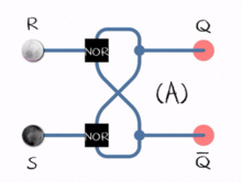
Consider a flip-flop circuit allowing for feedback, where the output does not only depend on the current input bits, but also on previous input bits; in other words, the computation maintains a “state” for its future inputs:
Such improved Boolean circuits are time-dependent, in the sense that a computation can be done on an unlimited chronological sequence of input bits, rather than on a finite set of input bits without any reference to its history. This gives us the intuition to disassemble a big, probably infinite string into a timely sequence and feed it into the machine, ask if it is accepted (or rejected). In this way, our ability to compute is no longer limited to finite languages. Circuits with states implement a sequential logic, and the resulting model of computation is often called a finite state machine (alternatively, a finite automaton). The language that can be decided by such a model of computation is the regular language, which is much more expressive than a finite language (i.e., a finite set of strings) since it can accommodate an infinite number of strings with a given pattern. Regular languages are of both theoretical and practical importance.
In my next post of this series, I will review the regular language and its corresponding models of DFAs/NFAs, as well as how to deal with regular expressions (which is much of a practical programming issue) from scratch. Then I’ll go down the Chomsky hierarchy and expand my collection of languages and their machines:
- Regular languages.
- Context-free languages.
- Context-sensitive languages.
- Recursive decidable languages.
- Presburger arithmetic and decidability.
- Recursively enumerable languages.
- Peano arithmetic and undecidability (Gödel’s incompleteness theorem).
- Turing machines and the halting problem. Church-Turing thesis.
5.1 More Circuits…
Despite their limited power of computation, Boolean circuits are yet a useful theoretical model when studying complexity theory, since it can be used to represent a specific computational mapping for given finite input bits (although not for the whole language). In a normal setting of computation, we construct a circuit that implements our desired mapping from input to output; however, the \(\textsf{CIRCUIT-SAT}\) (Boolean satisfiability) problem asks for a known circuit, whether there exists a set of input bits that evaluates to a certain output. Although we can easily show that this problem is decidable, no currently known algorithm can decide it efficiently (as it is proved to be NP-complete).
Naturally, we would also ask for a known circuit, whether we can correctly reverse any (or even all) input bits from its output. Generally it is not possible for decision problems, but if the number of output bits is the same as the number of input bits, or we can show that the information entropy contained in input is equal to the entropy contained in output, then things can be different. While we can construct a reversible circuit trivially, it is sometimes desirable to design a scheme of computation such that one can reverse input bits only with a secret key; while without the right key, reversing input from output must be as difficult as solving an instance of \(\textsf{CIRCUIT-SAT}\). These are very interesting topics of cryptography, where computational hardness assumptions form the theoretical basis for practical information security.
On the other hand, most Boolean logic gates we used are irreversible (except for a few like \(\lnot\)); this result may be shown using the concept of information entropy. However, in the research field of reversible computing, it is required that every step (gate) of the computation is perfectly reversible. An example of a nontrivial reversible gate is \(\textsf{XOR}_\textsf{reversible}(x, y) = (x, x \oplus y)\). By looking at its truth table, all possible outputs of 2-bit combinations \(\{(0, 0), (0, 1), (1, 0), (1, 1)\}\) appear with the same probability, so we can immediately tell that the output maintains the same entropy (2 bits) as the input does. Given any output \((x, x \oplus y)\), it is sufficient to reverse the input value \((x, y)\):
| \(x\) | \(y\) | Output \(x\) | Output \(x \oplus y\) |
|---|---|---|---|
| 0 | 0 | 0 | 0 |
| 0 | 1 | 0 | 1 |
| 1 | 0 | 1 | 1 |
| 1 | 1 | 1 | 0 |
The quantum counterpart of \(\textsf{XOR}_\textsf{reversible}\) is a controlled NOT gate (also CNOT), which is essential to the construction of quantum computers. Furthermore, as quantum circuits work in a probabilistic way, in contract to deterministic Boolean circuits, we are inspired to rethink of computation with an alternative mindset: From quantum circuits to finite automata, then quantum Turing machines and λ-calculus. Just because digital circuits are everywhere today and most of our software systems as well as programming languages work deterministically without any probable outcome, we should not easily take them for granted: What if quantum circuits were invented first, and how will computation be any different? After all, our abilities to compute are still bounded from two aspects: (1) Logically, Turing machines (and its equivalent models) cannot decide the halting problem, neither can its quantum counterpart do; (2) Physically, we can never implement a Turing machine of infinite memory, not even with a quantum computer, as restrained by the Bekenstein bound. Nevertheless, quantum computers are particularly of interest in complexity theory5, since designated algorithms that run on such circuits would allow us to attack many computationally hard problems in a more efficient, physically implementable way.
(To be continued.)
References
[1]Gödel, Kurt. 1931. “Über Formal Unentscheidbare Sätze Der Principia Mathematica Und Verwandter Systeme I.” Monatshefte Für Mathematik Und Physik 38 (1). Springer: 173–98.
[2]Pelletier, Francis Jeffry, Norman M. Martin, and others. 1990. “Post’s Functional Completeness Theorem.” Notre Dame Journal of Formal Logic 31 (3): 462–75.
[3]Shannon, Claude. 1948. “A Mathematical Theory of Communication.” Bell System Technical Journal 27 (4). Blackwell Publishing Ltd: 623–56. doi:10.1002/j.1538-7305.1948.tb00917.x. http://dx.doi.org/10.1002/j.1538-7305.1948.tb00917.x.
[4]Shannon, Claude, and others. 1949. “The Synthesis of Two-Terminal Switching Circuits.” Bell Labs Technical Journal 28 (1). Wiley Online Library: 59–98.
[5]Turing, Alan Mathison. 1937. “On Computable Numbers, with an Application to the Entscheidungsproblem.” Proceedings of the London Mathematical Society 2 (1). Wiley Online Library: 230–65.
In order to say things about general natural numbers and have a theory of basic arithmetic, we actually need a recursive language to accommodate such terms; that is beyond the scope of this article.↩
Also known as a Turing machine.↩
The complexity class of problems decidable by uniform Boolean circuits of polynomial size and polylogarithmic depth is \(\mathsf{NC}\). Such problems may also be decided efficiently on modern computers. However, it is an open question whether \(\mathsf{NC}=\mathsf{P}\).↩
I invented that word; it should be formally called recursively enumerable languages.↩
Due to the fact that quantum computers are probabilistic, we can only talk about \(\mathsf{BQP}\), which is the complexity class of problems that can be solved on a quantum computer in polynomial time with a bounded error probability of \(\frac{1}{3}\) for all instances. Its classical counterpart is \(\mathsf{BPP}\). But again, our knowledge about the relations among \(\mathsf{BQP}\), \(\mathsf{BPP}\), \(\mathsf{P}\) and \(\mathsf{NP}\) is woefully inadequate. Some believe that \(\mathsf{BQP} = \mathsf{NP}\), that is, every problem that can be decided by a nondeterministic Turing machine may also be decided by a quantum computer efficiently with only a bounded error probability; however this has not been proven yet.↩